
Introduction
Two organizations can both use Microsoft Fabric but require completely different capacities. One may have a small Power BI workload with occasional refreshes, completely satisfied by an entry-level capacity. Another organization may have hundreds of concurrent users, complex Power BI semantic models, heavy Data Factory pipelines, large scheduled transformations, AI workloads, and highly bursty enterprise reporting.
Choosing a Fabric SKU is not simply about picking the biggest capacity that fits the budget. It is a workload-sizing problem involving compute demand, concurrency, workload mix, burst behavior, utilization, growth, performance requirements, and cost. Understanding how Microsoft Fabric architecture distributes these compute demands across shared resources is essential before signing a capacity commitment.
The traditional approach of provisioning isolated compute for isolated services — a dedicated cluster for Spark, a dedicated pool for SQL, a dedicated premium capacity for Power BI — has been replaced by a pooled Capacity Unit (CU) model. Every workload draws from the exact same bucket. Consequently, capacity planning must shift from a siloed component estimation toward a unified demand model: Workload → CU demand → concurrency → headroom → SKU → cost → validation.
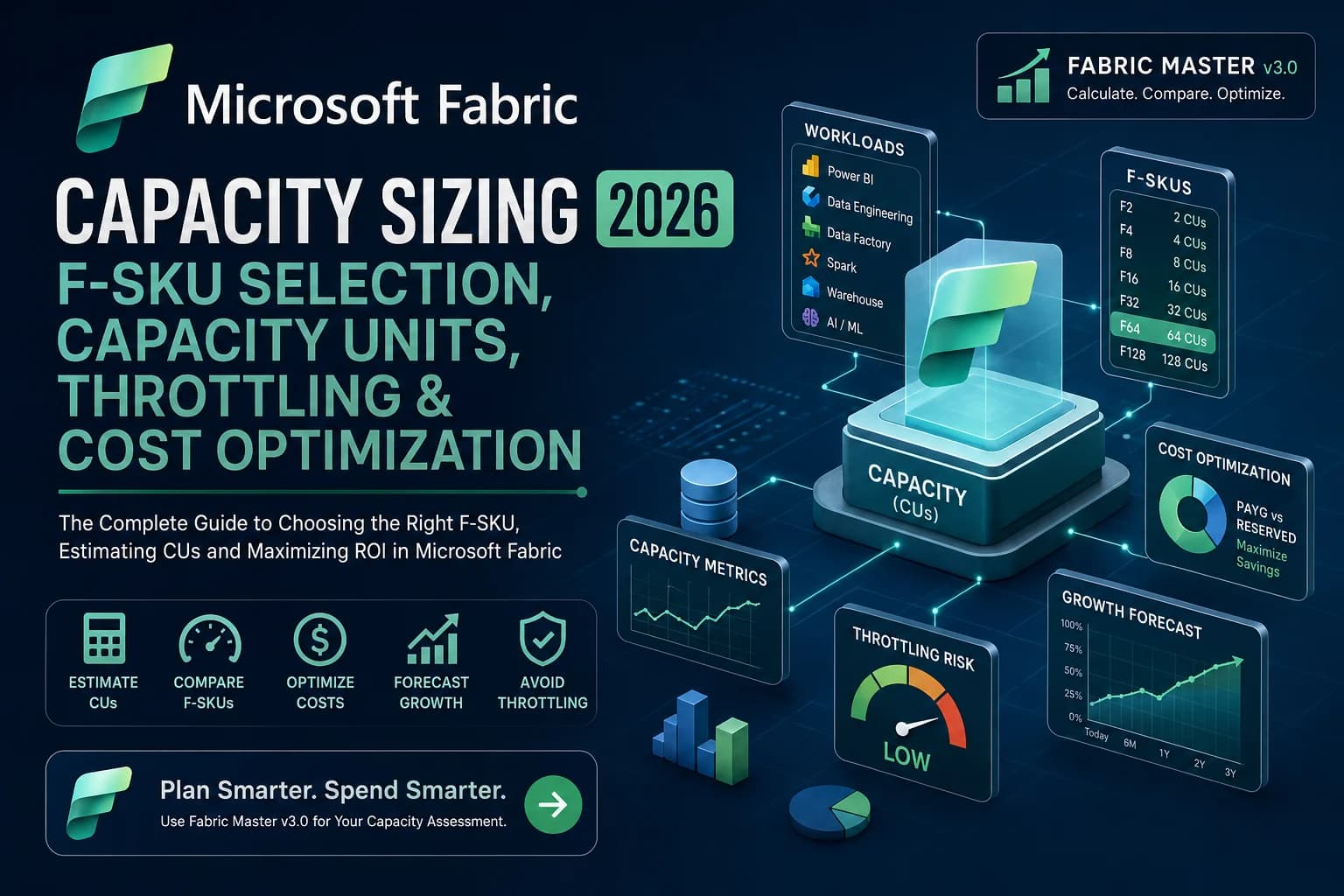
This article breaks down how to systematically size your Microsoft Fabric environment. A static SKU table is not enough. A basic calculator alone is not enough. We will explore how different engines consume CUs, how to plan for concurrency and headroom, what capacity throttling means in practice, and how to validate your modeled assumptions using production telemetry. Throughout the process, we will demonstrate how Fabric Master provides modeled estimation and decision support to accelerate this planning phase.
Table of Contents
- Executive Summary
- Quick Answer: Which F-SKU Should You Choose?
- What Is Microsoft Fabric Capacity?
- Capacity Units Explained
- How Fabric Capacity Sizing Actually Works
- Workload-by-Workload Sizing
- How Much Capacity Headroom Should You Keep?
- Fabric Capacity Throttling
- Validating with the Capacity Metrics App
- F-SKU Decision Table
- F32 vs F64: When Should You Upgrade?
- Capacity Sizing Example
- Capacity Sizing Is Also a FinOps Problem
- PAYG vs Reserved Pricing
- Optimization Before Resizing
- Calculate Your Fabric Capacity with Fabric Master
- Fabric Master Feature Mapping
- Frequently Asked Questions (FAQ)
Executive Summary
If you only have two minutes, here are the key takeaways for planning Microsoft Fabric capacity sizing:
- Capacity sizing is workload-specific: User counts alone cannot determine your SKU. You must evaluate the intensity of Spark, SQL, and Power BI workloads.
- Capacity Units are the core compute measurement: Every operation burns a predictable fraction of CUs based on execution time and intensity.
- F-SKU selection should reflect workload demand: Choose a SKU based on concurrent demand plus buffer, not simply average utilization.
- Average utilization can hide peaks: Designing a capacity purely on average daily consumption will lead to severe performance degradation during concurrent spikes.
- Concurrency matters: Ten users querying large semantic models simultaneously demand exponentially more instantaneous CUs than ten users spread across the day.
- Headroom matters: Planning for 100% baseline utilization leaves zero room for burst operations, growth, or unexpected workload scheduling collisions.
- Throttling is a signal, not merely a pricing issue: Interactive rejection or background delays indicate either a need for workload optimization or a larger SKU.
- Production telemetry should validate modeled estimates: Modeled estimates must eventually be validated against actual usage.
- Workload optimization can sometimes be better than scaling: Tuning a poorly designed Fabric Warehouse workload is often cheaper and more effective than upgrading from F64 to F128.
- Fabric Master can provide an initial modeled assessment: Use Fabric Master to generate initial estimates based on workload assumptions.
- Microsoft Capacity Metrics should validate production usage: Microsoft's official app remains the definitive source for real-world CU burn and throttling diagnosis.
Quick Answer: Which Fabric F-SKU Should You Choose?
A common mistake is seeking a definitive mapping of "X users equals SKU Y." SKU selection cannot be determined reliably from user count alone because 100 casual report viewers require vastly less compute than 5 data engineers compiling massive Apache Spark transformations. However, a general directional framework based on workload profiles provides a starting point:
- Small workload (F2–F8): May be appropriate for lightweight, departmental reporting with minimal background transformation. Suitable for Dev/Test environments or small teams relying primarily on scheduled Power BI refresh without heavy concurrency.
- Growing departmental workload (F8–F16): Fits mid-sized teams running moderate Data Factory pipelines and interactive dashboards. Concurrency is limited, and heavy Spark jobs should be strictly scheduled during off-peak hours.
- Medium enterprise workload (F16–F32): Suitable for organizations running active data warehouses, regular semantic model processing, and consistent interactive querying across multiple departments. Supports more aggressive background transformations without immediately starving interactive performance.
- High-concurrency / multi-workload enterprise (F32–F64+): The entry point for complex enterprise architectures running concurrent Spark jobs, continuous Data Factory orchestration, massive warehouse queries, and hundreds of interactive Power BI users. F64 is notably the tier where Power BI Free users can consume content without individual Pro licenses.
- Large enterprise (F128+): Necessary for vast architectures requiring high-throughput capacity planning for Fabric workloads spread across global teams, near real-time streaming pipelines, and thousands of concurrent interactive sessions.
If you are unsure where your workload fits, use the Fabric capacity calculator within Fabric Master to model specific engine assumptions before provisioning.
What Is Microsoft Fabric Capacity?
In Microsoft Fabric, capacity refers to a dedicated pool of compute resources allocated to your tenant. Instead of provisioning an isolated virtual machine for your database and a separate cluster for your data integration, Fabric utilizes a shared compute model. Every workload — whether a Spark notebook execution, a SQL warehouse query, or a Power BI dashboard render — draws computing power from this shared pool.
This compute power is quantified in Capacity Units (CUs). When you purchase Fabric, you purchase a specific F-SKU, which guarantees a continuous baseline of CUs available to all workspaces assigned to that capacity. When a workload executes, it consumes a fraction of those CUs based on the intensity and duration of the operation.
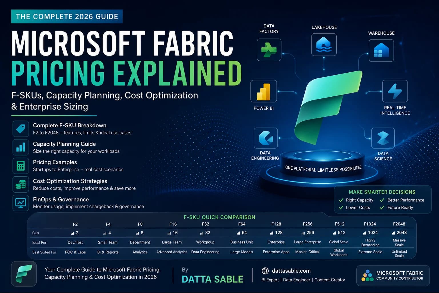
| SKU | Capacity Units (CUs) | Typical Planning Context | Important Caveat |
|---|---|---|---|
| F2 | 2 | Dev/Test environments, small POCs | Will severely throttle under concurrent load. |
| F4 | 4 | Small departmental reporting | Avoid running heavy Spark and Warehouse workloads simultaneously. |
| F8 | 8 | Moderate analytical pipelines | Scheduled backgrounds tasks must be carefully orchestrated. |
| F16 | 16 | Mid-market standard analytics | Capable of decent parallelism but watch out for peak concurrency. |
| F32 | 32 | Medium enterprise multi-engine architecture | A common baseline for significant production deployments. |
| F64 | 64 | High-concurrency enterprise workloads | Enables Power BI Free user consumption. |
| F128 | 128 | Large enterprise global scale | Typically requires splitting workspaces logically to isolate critical workloads. |
Capacity Units Explained
A Capacity Unit (CU) is the standardized measure of compute power in Fabric. If you provision an F64 SKU, you receive 64 seconds of compute capacity every single second.
Fabric calculates consumption through continuous evaluation periods. When a workload executes, Microsoft calculates the actual computational effort required (CPU seconds, memory footprint, data scanned) and translates it into a CU consumption metric. Because modern analytics workloads are inherently "bursty" — requiring massive compute for a few seconds and then sitting idle — Fabric employs an intelligent smoothing mechanism.
Smoothing takes a massive spike in compute (a burst) and averages the CU consumption over a longer time window (e.g., 24 hours for background operations, shorter intervals for interactive queries). This allows a relatively small capacity to process a massive, instantaneous job without immediately throttling, by effectively borrowing against future idle capacity.
Illustrative Example: If a scheduled Spark job demands 200 CUs for 1 minute, but you only have an F64 capacity, smoothing spreads that massive 200 CU burn rate out over the next 24 hours, registering as a tiny fractional CU burn per minute. The job finishes fast, but your capacity "pays off" the compute debt gradually. However, if you continuously burst without idle periods, your smoothed average will eventually exceed your baseline 64 CUs, leading to throttling.
This is why "64 CUs" does not equal "64 users." A single user running a catastrophically complex Data Factory pipeline could theoretically exhaust an F64 if they run it continuously, while 64 casual users viewing cached Power BI reports might barely register a blip on an F8.
How Fabric Capacity Sizing Actually Works
To avoid the trap of guessing a SKU based on user count, adopt a structured sizing methodology.
Dattasable Capacity Sizing Framework
- Inventory workloads: Catalog all planned Spark jobs, SQL queries, Data Factory pipelines, and Power BI models.
- Estimate baseline demand: Determine the average CU consumption required for steady-state operations.
- Identify peak periods: Pinpoint when scheduled data loads intersect with high interactive usage (e.g., Monday 8:00 AM).
- Model concurrency: Calculate the impact of multiple users hitting the Warehouse or Semantic Models simultaneously.
- Account for burst workloads: Acknowledge that smoothing handles short bursts, but continuous bursts require raw capacity.
- Add growth assumptions: Factor in expected data volume increases and new user onboarding over the next 12-18 months.
- Define acceptable headroom: Decide the maximum utilization threshold before performance risks become unacceptable (e.g., targeting 70% peak utilization).
- Evaluate throttling risk: Assess what happens to business operations if background rejection or interactive delays occur.
- Compare candidate SKUs: Map the resulting CU requirement to the closest F-SKU.
- Validate with production telemetry: Monitor the Microsoft Fabric Capacity Metrics app post-deployment.
- Reassess periodically: Treat sizing as a continuous FinOps cycle, not a one-time event.
    flowchart TD
      WorkloadInventory[Workload Inventory] --> BaselineDemand[Baseline Demand]
      BaselineDemand --> PeakDemand[Peak Demand]
      PeakDemand --> Concurrency[Concurrency]
      Concurrency --> Headroom[Headroom]
      Headroom --> CandidateSKU[Candidate F-SKU]
      CandidateSKU --> CostEval[Cost Evaluation]
      CostEval --> ProdValidation[Production Validation]
Workload-by-Workload Sizing
Power BI / Semantic Models
Power BI represents the visualization and semantic modeling layer. Interactive report usage consumes interactive CUs, while scheduled refreshes consume background CUs. Concurrency is a massive factor here: 100 executives viewing an executive dashboard at exactly 9:00 AM generates a spike in query processing. The underlying model architecture fundamentally dictates consumption. Complex DAX running against an Import model behaves differently than a Direct Lake setup. Proper tuning for Direct Lake performance ensures optimal paging of Delta Parquet columns into memory, reducing sustained CU demand compared to heavy DirectQuery models which push compute down to the underlying SQL engine.
Data Factory
Data Factory handles pipeline orchestration and data movement. Scheduled background workloads are smoothed over 24 hours, meaning heavy nightly ETL pipelines can often run on relatively small capacities without impacting daytime interactive performance. However, high-concurrency pipeline execution or continuously running micro-batches will aggregate and steadily raise the baseline utilization.
Spark
Spark notebooks and batch processing jobs are notorious for bursty compute. Spark can autoscale to consume massive amounts of compute very quickly to process large data volumes. While smoothed, a poorly optimized Spark job that scans excessive partitions can artificially inflate CU consumption. The Spark CU estimator in Fabric Master can help model the impact of node sizing and execution time.
Warehouse
Fabric’s distributed T-SQL engine provides relational data warehousing capabilities. SQL workloads consume CUs during concurrent queries, complex joins, and heavy ingestion transformations. Every BI consumption query directed at the warehouse utilizes CUs. Unoptimized queries scanning massive fact tables without proper filtering will burn CUs aggressively.
    flowchart TD
      PBI[Power BI]
      DF[Data Factory]
      SPK[Spark]
      WH[Warehouse]
      AI[AI Functions]

      PBI --> SharedCap
      DF --> SharedCap
      SPK --> SharedCap
      WH --> SharedCap
      AI --> SharedCap

      SharedCap((Shared Fabric Capacity)) --> CUConsume[CU Consumption]
      CUConsume --> Util[Utilization]
      Util --> Perf[Performance / Throttling]
Calculate Your Fabric Capacity
How Much Capacity Headroom Should You Keep?
A common misconception is that a capacity should target 100% utilization to maximize return on investment. Designing for 100% average utilization is functionally guaranteeing failure during peak periods. Headroom is not wasted compute; it is the operational shock absorber for your data platform.
Headroom absorbs unexpected bursts (e.g., an analyst runs a massive ad-hoc query), manages scheduling collisions (when a pipeline runs long and overlaps with early morning BI usage), and provides a buffer for natural organic growth before requiring a formal FinOps approval for an SKU upgrade.
    flowchart TD
      subgraph Dattasable Capacity Headroom Model
      Base[Baseline Demand] --> Plus1(+)
      Plus1 --> Peak[Peak Demand]
      Peak --> Plus2(+)
      Plus2 --> Burst[Burst Buffer]
      Burst --> Plus3(+)
      Plus3 --> Growth[Growth Buffer]
      Growth --> Equals(=)
      Equals --> PlanReq[Planning Requirement]
      end
Dattasable planning model
Dattasable recommendation: Treat sustained peak utilization, workload concurrency, and growth headroom as separate planning dimensions rather than sizing from average utilization alone. Targeting roughly 70-80% utilization during known peak windows provides a sensible safety margin.
Fabric Capacity Throttling
When a capacity's smoothed CU consumption exceeds 100% of its provisioned limit, it enters capacity pressure. To protect the underlying service infrastructure and enforce the SKU limits, Microsoft Fabric initiates throttling.
Throttling applies in stages based on the severity of the overage:
- Interactive Delay: The first stage. Interactive operations (like a user clicking a Power BI visual or running a T-SQL query) are intentionally delayed. The system makes the request wait before execution.
- Interactive Rejection: If pressure worsens, Fabric will flatly reject new interactive requests. Users receive errors indicating the capacity is overloaded.
- Background Rejection: The most severe stage. Even background operations (like scheduled Data Factory pipelines or Semantic Model refreshes) are rejected and fail to run.
Fabric utilizes a "carryforward" mechanism. If you burn 200% of your capacity in one hour, the debt is carried forward. You must burn down this debt before full performance is restored. Persistent throttling indicates a fundamental architectural issue: you must optimize workloads, reschedule heavy jobs to off-peak hours, distribute workloads, increase capacity, or re-evaluate your entire capacity architecture.
Crucial distinction: Poor query performance is not automatically caused by capacity throttling. A poorly written query on an idle F128 will still be slow. Always diagnose the workload before assuming throttling is the culprit.
    flowchart LR
      PerfIssue[Performance issue] --> CheckMetrics[Check Metrics]
      CheckMetrics --> Identify[Identify workload]
      Identify --> CheckUtil[Check utilization]
      CheckUtil --> CheckThrot[Check throttling]
      CheckThrot --> Opt[Optimize workload]
      Opt --> Rebal[Rebalance]
      Rebal --> Resize[Resize if required]
      Resize --> Mon[Monitor again]
How to Validate Your Capacity Size Using the Microsoft Fabric Capacity Metrics App
Microsoft documents the Capacity Metrics app as a mechanism for monitoring utilization and informing sizing decisions. It is the absolute source of truth for production telemetry.
The practical validation loop involves:
- Establish workload: Deploy your analytical solutions to the capacity.
- Observe utilization: Use the Compute tab to monitor CU consumption trends over 14 days.
- Identify peak timepoints: Locate the highest spikes in utilization.
- Drill into operations: Use the Timepoint item detail drill-down to see exact interactive vs. background breakdown.
- Identify top consumers: Find the specific item (e.g., an inefficient Notebook or semantic model) driving the burn.
- Inspect throttling: Review the throttling information to see if delays or rejections have actively occurred.
- Compare against SKU: Determine if your baseline + headroom comfortably fits the F-SKU.
- Resize if justified: Scale up or down based on hard evidence.
- Monitor again: Repeat the cycle.
F-SKU Decision Table
| SKU | CUs | Best-fit scenario | Typical workload profile | Growth considerations | Warning signs that you may have outgrown it |
|---|---|---|---|---|---|
| F2 | 2 | POCs, Dev/Test | Very light Power BI Import refreshes | Scales poorly with any heavy data volumes | Frequent background rejections when testing Spark. |
| F4 | 4 | Small isolated reporting | Scheduled ELT and simple semantic models | Cannot handle complex concurrent background jobs | Struggles with large Direct Lake paging. |
| F8 | 8 | Departmental workloads | Moderate analytical pipelines | Limited by concurrency peaks | Long-running data factory pipelines causing interactive lag. |
| F16 | 16 | SME data platforms | Standard Warehouse queries, steady pipelines | Provides buffer for increasing report concurrency | Interactive delays during morning peak login windows. |
| F32 | 32 | Medium enterprise multi-engine architecture | Regular scheduled pipelines and heavy queries | Good baseline for robust ELT, but watch concurrency | Heavy Spark jobs eating into Power BI reporting CUs. |
| F64 | 64 | Enterprise baseline, Free user report sharing | Heavy Direct Lake models, concurrent Spark | Solid baseline for onboarding new business units | Sustained 90%+ utilization preventing new workloads. |
| F128 | 128 | Large-scale global enterprise operations | Massive KQL streaming, continuous ETL | Consider splitting into multiple capacities by domain | Cost overhead outweighs the benefits of a single unified pool. |
F32 vs F64: When Should You Upgrade?
The jump from F32 to F64 is the most critical decision point in Fabric capacity planning. F64 is the tier that unlocks Power BI Free user consumption (comparable to the old Power BI Premium P1 tier). However, beyond licensing, the compute difference is vast.
You should upgrade from F32 to F64 when your workload intensity shifts from "departmental scheduled pipelines" to "enterprise continuous processing." If your Spark jobs require higher node counts for efficient parallelism, or if your Data Factory pipelines consistently collide with interactive Power BI users causing throttling, F64 provides the necessary compute depth to absorb these continuous shocks.
Warehouse workloads particularly benefit from F64 when concurrent complex queries are running. Heavy Direct Lake architectures similarly benefit when caching large datasets. If growth forecasting shows your F32 exceeding 80% baseline utilization, an upgrade is prudent.
Capacity Sizing Example
Imagine a fictional enterprise, Contoso Financial, evaluating Fabric. Their workload consists of high-concurrency Power BI interactive usage, massive overnight semantic model refreshes, continuous Data Factory pipelines, heavy Warehouse query patterns at month-end close, and some Spark jobs for forecasting.
Illustrative Dattasable sizing example:
- Baseline: 15 CUs continuous demand for background orchestration.
- Peak: +25 CUs required during the 9:00 AM interactive login rush and month-end close overlap.
- Concurrency Buffer: +10 CUs to handle simultaneous complex DAX queries.
- Headroom & Growth: +14 CUs for unexpected bursts and next year's onboarding.
- Total Planning Requirement: 64 CUs.
This structured approach directs Contoso firmly toward an F64 SKU, ensuring stability during month-end close without flying blind into throttling.
Capacity Sizing Is Also a FinOps Problem
Capacity planning and cost management are fundamentally linked. Over-provisioning wastes budget, while under-provisioning destroys user trust through poor performance. Effective FinOps in Fabric requires right-sizing the capacity, optimizing workload schedules (moving heavy ETL to weekends or nights where smoothing handles the load), and potentially separating workloads into multiple capacities (e.g., an F32 for production ELT and an F16 for Dev/Test) to isolate noisy neighbors and enact capacity consolidation.
For a comprehensive look at the financial models underlying these decisions, review our Microsoft Fabric pricing and capacity planning guide.
Estimate Fabric Capacity Costs
PAYG vs Reserved Pricing
Fabric Capacities can be purchased via Pay-As-You-Go (PAYG) or Reserved Instances (typically a 1-year commitment horizon). PAYG is highly flexible—you can pause it or scale it dynamically, making it excellent for unpredictable workloads or short-term POCs. Reserved Instances require an upfront or monthly commitment but offer significantly lower effective hourly rates. The break-even point often heavily favors Reserved Instances if a capacity runs 24/7 for steady-state workloads. Evaluate your commitment horizons carefully using our Fabric reserved savings calculator.
Don't Scale the Capacity Before You Diagnose the Workload
Scaling up from F64 to F128 doubles your compute, but it also roughly doubles your cost. Before requesting a budget increase, enforce this troubleshooting checklist:
- Are inefficient queries draining resources?
- Are Power BI models suffering from poor semantic model design (e.g., high-cardinality unused columns)?
- Are you running an excessive refresh frequency?
- Are Warehouse queries performing excessive full table scans instead of leveraging partitioning?
- Are Data Factory pipelines scheduled simultaneously, causing massive scheduling collisions?
- Are Spark jobs configured with massive driver nodes for tiny data manipulations?
- Can you implement better workload distribution?
Optimization before scaling is a golden rule in FinOps.
Calculate Your Fabric Capacity Requirement with Fabric Master
Fabric Master v3.0 is an independent workload modeling, capacity planning, FinOps and decision-support platform designed specifically for Microsoft Fabric architects. It helps you translate abstract workloads into concrete F-SKU recommendations.
Important Note: Fabric Master provides a modeled assessment based on the workload assumptions entered by the user. Production decisions should always be validated against Microsoft Fabric Capacity Metrics and actual telemetry.
    flowchart LR
      Inputs[User Inputs] --> Model[Workload Model]
      Model --> CUEst[CU Estimate]
      CUEst --> Cands[F-SKU Candidates]
      Cands --> Cost[Cost Model]
      Cost --> Growth[Growth Forecast]
      Growth --> Rec[Recommendation]
      Rec --> PDF[PDF Assessment]
      PDF --> Prod[Production Validation]
Fabric Master Feature Mapping
| Planning Need | Fabric Master Capability |
|---|---|
| Capacity sizing | Capacity Calculator |
| F-SKU selection | F-SKU Comparison |
| Cost estimation | Cost Estimator |
| Reserved pricing | Reserved Savings |
| Spark workloads | Spark CU Estimator |
| Power BI | Power BI Capacity planning |
| Enterprise assessment | Capacity Consultant |
| PDF reporting | Assessment Report |
| Pricing | Global Pricing Matrix |
Frequently Asked Questions (FAQ)
- What is Microsoft Fabric capacity sizing?
- It is the process of evaluating compute demand across Spark, SQL, Power BI, and integration workloads to select an appropriate F-SKU that prevents throttling while managing costs.
- How are Capacity Units used in Fabric?
- Capacity Units (CUs) represent the shared compute pool. Every workload consumes a fraction of these CUs based on processing intensity, and background bursts are smoothed over time.
- How do I choose a Fabric F-SKU?
- Catalog your workloads, model peak concurrency, define headroom for growth, and evaluate throttling risks, then map that requirement to a specific tier (e.g., F32 vs F64).
- Is F32 enough for Microsoft Fabric?
- F32 is excellent for medium enterprise workloads, but lacks the Power BI Free user consumption capabilities of F64. If your organization relies heavily on free report viewers, F64 is typically the baseline.
- When should I move from F32 to F64?
- Upgrade when background tasks consistently collide with interactive queries, causing sustained throttling, or when you need Power BI free user viewing capabilities.
- What causes Fabric capacity throttling?
- Throttling occurs when the smoothed CU consumption exceeds the capacity's limit. This triggers interactive delays, interactive rejections, and eventually background job failures.
- How much headroom should I keep?
- Aim for roughly 70-80% peak utilization. The remaining 20-30% acts as an operational buffer against unexpected spikes and concurrent organic growth.
- Can Fabric Master calculate my required capacity?
- Yes, Fabric Master provides comprehensive modeling tools to estimate CU consumption across various workload assumptions.
- Is Fabric Master an official Microsoft sizing tool?
- No, Fabric Master is an independent decision-support platform. All modeled estimates must be validated against actual production telemetry via the Microsoft Capacity Metrics app.
- How should I validate a capacity recommendation?
- Use the Microsoft Fabric Capacity Metrics app over a realistic 14-day cycle, analyzing peak timepoints and identifying top CU consumers to verify the modeled estimate.
- What is the difference between PAYG and Reserved capacity?
- PAYG (Pay-As-You-Go) is flexible and can be paused, suitable for ad-hoc processing. Reserved instances involve a term commitment (e.g., 1 year) in exchange for significantly reduced hourly rates.
- Can workload optimization reduce the required Fabric SKU?
- Absolutely. Tuning DAX models, optimizing T-SQL queries, and properly sizing Spark nodes can drastically reduce CU burn, avoiding expensive SKU upgrades.